

View on GitHub
Open this notebook in GitHub to run it yourself
Cybersecurity Vertex Cover Patch Management Challenge for Tackling Kill Chains
This tutorial is based on work submitted by Mark Carney in November 2022 [1]. The Min Vertex Cover (MVC) problem is a classical issue in graph theory and computer science, which aims to find a minimum set of vertices where each edge of the graph is incident to at least one vertex in the set. Vulnerability graphs (related to attack graphs) showcase a method for solving significant cybersecurity problems with quantum computing using Classiq. This tutorial suggests a method to prioritize patches by expressing the connectivity of various vulnerabilities on a network with a QUBO, then solving this with Classiq. Such a solution has the potential to effectively remove significant kill chains (paths to security compromise) within a given network leveraging a quantum computer.Introduction
Patch management is a common pain point for large-scale enterprises or widely distributed systems such as smartphones or IoT devices. Indeed, the lack of appropriate patching is indicated as a central cause for some high profile cybersecurity breaches. A variety of approaches have been proposed to improve the categorization and management of patches, including deep learning technologies. This tutorial suggests a method of prioritizing patch management by analyzing vulnerability data on assets as a bipartite graph. Given that attacks are composed of ‘kill chains’—which themselves comprise sequences of exploits leveraging vulnerabilities (that are coincident in our model)—this process suggests disconnecting vulnerability sequences, thereby significantly reducing potential kill chains in a given network. This challenge, however, involves a known NP-hard problem. Leveraging quantum computation and optimization methods for vulnerability analysis of this kind opens new avenues of optimization of cybersecurity and related data for consideration.The tutorial presents a method of prioritizing the patching of vulnerabilities by considering their connectivity and solving them using Classiq.
Bipartite Graph Representation
The heart of the methodology represents vulnerabilities and assets as nodes in a bipartite graph. Useful terminology:Kill Chains
A ‘kill chain’ is a multi-stage sequence of events that leads to the compromise of a network. Many of the examples of kill chains involve sequences of vulnerabilities, with the sequence dependent on the assets that intersect these vulnerabilities. Vulnerabilities: Weaknesses in the system that result from an error in the design, implementation, or configuration of the operating system or an application software. Assets: Items with value; for example, data stored in the system. The availability, consistency, and integrity of assets are to be preserved.Attack Graphs
‘Attack graphs’ feature in some interesting approaches to managing and mitigating security threats. They provide ways of analyzing network-oriented vulnerability data that many cybersecurity information sources generate. Attack graphs are labeled transition systems that model adversary capabilities within a network and how they can be elevated by transitioning to new states via the exploitation of vulnerabilities (e.g., a weak password, a bug in a software package, or the ability to guess a stack address). Attack graphs can discover paths that an adversary may use to escalate his privileges to compromise a given target (e.g., customer database or an administrator account). These sequences of possible vulnerabilities and asset pathways are commonly known as “kill chains.” Kill chains depict comprehensive attack scenarios that outline the steps taken to target a specific critical asset.Attack graph example
Vulnerability Graphs
A theoretical way of analyzing vulnerabilities on a computer network uses ‘vulnerability graphs’, derived from the notion of ‘attack graphs’. A graph ; with a set of vertices and a set of edges , comprises pairs of elements from . A bipartite graph is a graph with a partition of into two sets such that , and . A vulnerability graph is a bipartite graph where one partition of vertices represents network assets and the other represents vulnerabilities. The edges of represent a given asset affected by a detected vulnerability. A kill chain is a sequence of vertices from the vulnerability partition of a vulnerability graph such that for each there exists at least one asset with .- Whilst the formulation in utilities directed graphs, for simplicity this tutorial uses undirected simple graphs to represent the same data.
- Note the lack of any information coded about severity ratings for vulnerabilities, e.g., CVSS scores.
Connectivity Dual Graphs
The dual graph is constructed as follows. For each vulnerability vertex for :- Add to if .
- Enumerate a list of asset vertices connected to .
- Iterating over this list of assets, for each connected to each host :
- Add to .
- Add to .
- If already exists, add 1 to the weight of that edge.
- Remove from and continue with .
Removing Kill Chains with Vertex Covers
Removing the vertices in a vertex cover on from leaves V totally disconnected on the vulnerability partition to itself via the host partition. Removing every ‘vulnerability-host-vulnerability’ sub-path in a vulnerability graph by means of a minimum vertex cover on , removes a significant number of kill chains found in the paths of .Min Vertex Cover: Mathematical Formulation
The MVC problem can be formulated as an Integer Linear Program (ILP): Minimize: Subject to and where- is a binary variable that equals 1 if node is in the cover and 0 otherwise
- is the set of all edges (connected and not connected)
- is the set of vertices in the graph
By utilizing a quantum computing setup, you can efficiently solve an NP-hard problem, reducing the time required to find the most at-risk vulnerabilities and patching them with more priority.You can run iterations over security data more effectively with feedback from new information, thereby improving security.
Toy Network Example
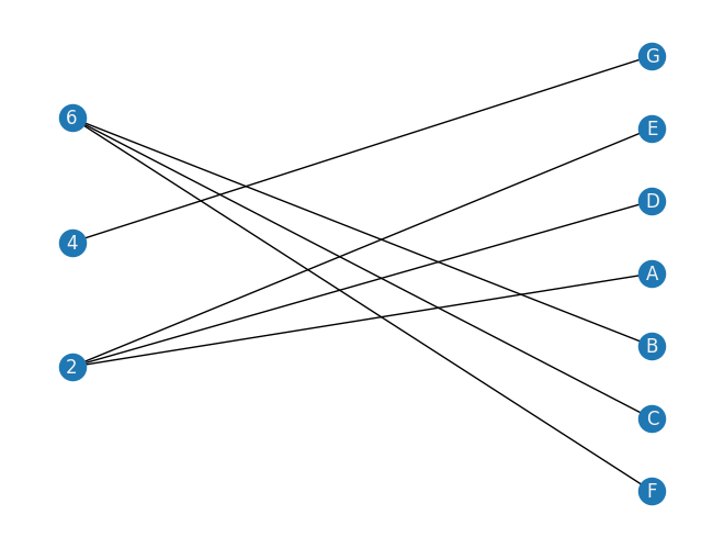
The following vulnerability graph has assets to and vulnerabilities through :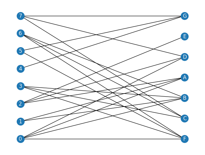
Above is the bipartite graph with vulnerabilities on the left and assets on the right.
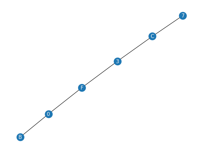
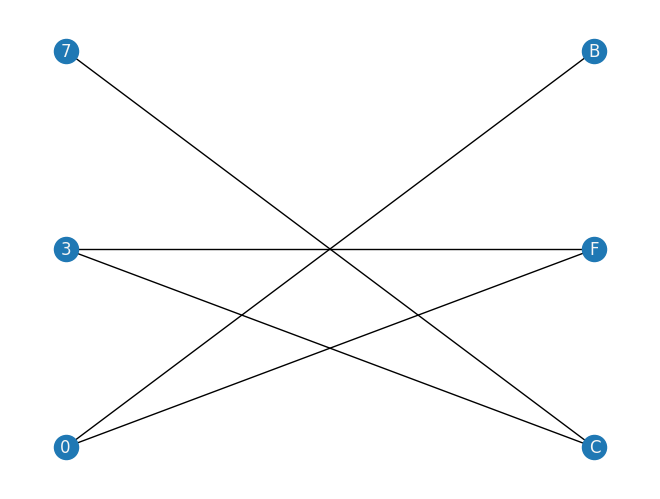
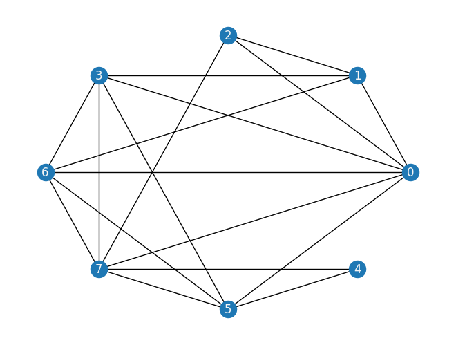
Above is the dual graph for solving the MVC.
Building the Optimization Model from Graph Input
To build the optimization model, use Pyomo, which is a Python-based, open-source optimization modeling language with a diverse set of optimization capabilities. Formalize the QUBO model into a Pyomo model object. Classiq seamlessly incorporates the Pyomo object into its model. Define the Pyomo model for building a Classiq model using the mathematical formulation defined above:- a binary variable declaration for each node (model.x) indicating whether the variable is chosen for the set.
- a constraint rule ensuring that all edges are covered.
- an objective rule that minimizes the number of selected nodes.
Output:
Solving MVC with Classiq and QAOA
Follow the steps of solving the problem with Classiq using the Quantum Approximate Optimization Algorithm (QAOA) [2]. QAOA is a quantum algorithm designed to solve combinatorial optimization problems, making it an ideal candidate for tackling the MVC problem in large scale WSNs. Apply QAOA to the modeled graph, iteratively adjusting the parameters to navigate the solution space and identify the MVC. Quantum computing’s unique ability to explore multiple solution candidates simultaneously accelerates the optimization process, significantly outperforming classical algorithms for complex problems. To solve the Patching Prioritization Problem with Classiq:- Build a Classiq model
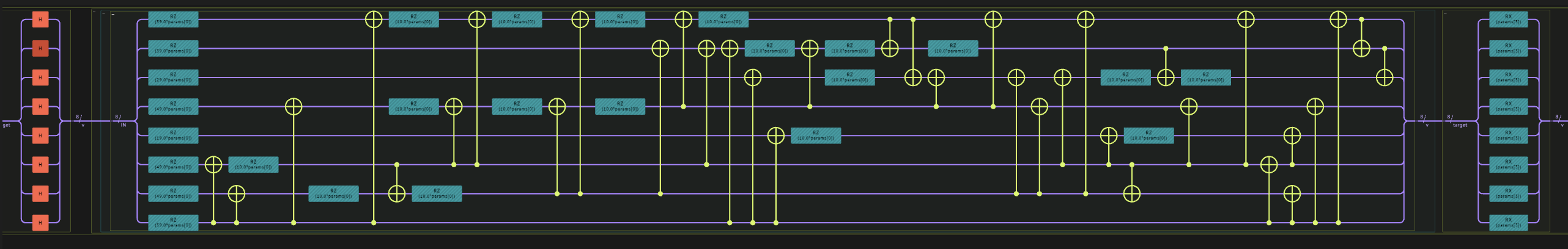
- Generate a parameterized quantum circuit
- Execute the circuit and optimize the parameters to get the optimal solution
- Building a Classiq Model
num_layers):
That’s it! Your Classiq model is all set!!
- Generating a Parameterized Quantum Circuit
Output:
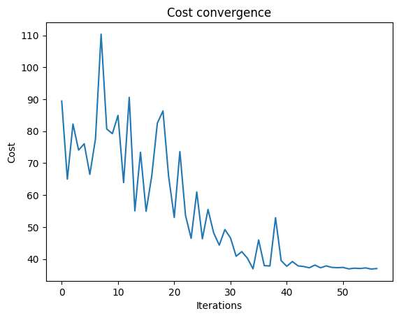
- Executing the Circuit: Optimizing Parameters to Get the Optimal Solution
optimize method of the CombinatorialProblem object.
For the classical optimization part of the QAOA algorithm we define the maximum number of classical iterations (maxiter) and the -parameter (quantile) for running CVaR-QAOA, an improved variation of the QAOA algorithm [3].
- Analyzing the Execution Results
Output:
sample method:
| solution | probability | cost | |
|---|---|---|---|
| 112 | {‘x’: [1, 1, 0, 1, 0, 1, 0, 1]} | 0.001465 | 5 |
| 115 | {‘x’: [1, 1, 0, 0, 0, 1, 1, 1]} | 0.001465 | 5 |
| 55 | {‘x’: [1, 1, 1, 0, 0, 1, 1, 1]} | 0.003906 | 6 |
| 2 | {‘x’: [1, 0, 1, 1, 1, 1, 1, 0]} | 0.056152 | 6 |
| 178 | {‘x’: [1, 1, 0, 1, 1, 0, 1, 1]} | 0.000488 | 6 |
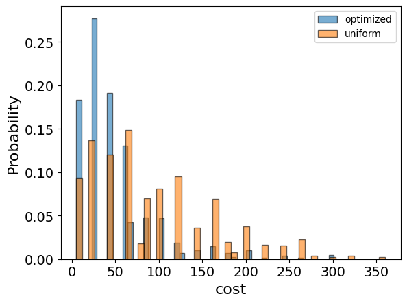

You obtained a set of vertices that form the minimum vertex cover.
Given that the MVCV vulnerability nodes are patched, the rest of the vulnerabilities are disconnected from one other.This significantly breaks most of the network kill chains.
Larger Scale Models
TBDThe leveraging of short term solutions for NP-hard problems that are present in cybersecurity data is a potentially rich vein of exciting possibilities.The fast and efficient resolution of cybersecurity data problems also helps reduce the analysis and reaction times of security teams.
References
[1] [Cutting Medusa’s Path -- Tackling Kill-Chains with Quantum Computing.](https://arxiv.org/abs/2211.13740)