
View on GitHub

Open this notebook in GitHub to run it yourself

Oblivious Amplitude Amplification

This demo explains the Oblivious Amplitude Amplification algorithm (OAA) [2], which can be used as a building block in algorithms such as Hamiltonian simulations. We start with a short recap, then show how to use it in conjunction with the Linear Combination of Unitaries (LCU) algorithm.

Problem formulation

  • Input: A (s,l,0)(s, l, 0)-block-encoding WW of a matrix UU.
  • Promise: UU is unitary (or close to unitary).
  • Output: A (1,l,0)(1, l, 0)-block-encoding of UU.

Background

Recap: Amplitude Amplification

Ref. [1] shows how to use the Grover operator to amplify a specific state. In detail, given a unitary AA to prepare a state ψ|\psi\rangle: A0=ψ=aψ0+1a2ψ1A|0\rangle = |\psi\rangle = a|\psi_0\rangle + \sqrt{1-a^2}|\psi_1\rangle and a unitary Rψ1R_{\psi_1} to implement a reflection over the state ψ1\psi_1: Rψ1(aψ0+1a2ψ1)=aψ01a2ψ1R_{\psi_1}(a|\psi_0\rangle + \sqrt{1-a^2}|\psi_1\rangle) = a|\psi_0\rangle - \sqrt{1-a^2}|\psi_1\rangle We want to decrease the amplitude of ψ1\psi_1 to be
ψ0|\psi_0\rangle, ψ1|\psi_1\rangle define a two-dimensional subspace where the applications of the Grover operator are effectively rotations. To do that we also need to do a reflection about the initial state ψ|\psi\rangle: Sψ=AR0AS_\psi = AR_0A^{\dagger} where R0R_0 is a reflection about the 0|0\rangle state. The rotations can be used to take the initial vector ψ|\psi\rangle closer to ψ0|\psi_0\rangle. image.png

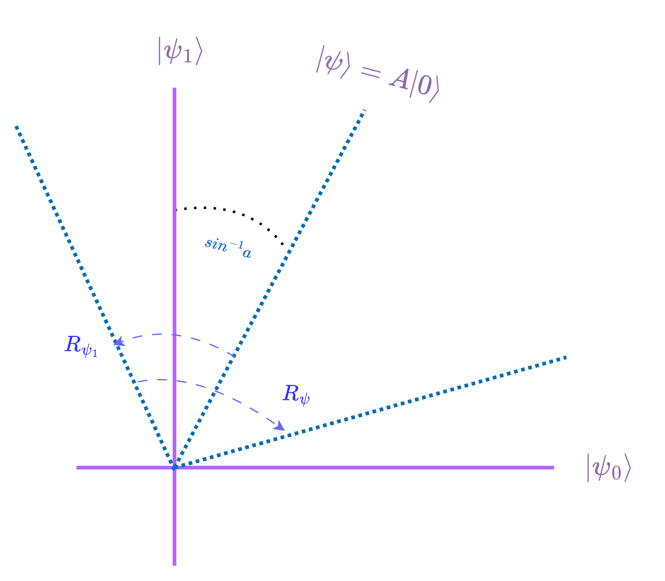
Why Another Version?

As you might have noticed, the amplification requires the “recipe” AA for the preparation of ψ\psi, and uses it to perform the reflection around the initial state. In certain scenarios, such as in Hamiltonian simulations, we might not be able to create the initial state or it is very inefficient. Specifically, we look at a (s,l,0)(s, l, 0)-block-encoding WW of a matrix UU: W0lψ=1s0lUψ+11s2ϕW|0^l\rangle|\psi\rangle = \frac{1}{s}|0^l\rangle U|\psi\rangle + \sqrt{1-\frac{1}{s^2}}|\phi\rangle (For detailed explanations of block-encodings and Hamiltonian simulations, see this demo.) We want to amplify the amplitude of the state that is in the block, i.e., 0lUψ|0^l\rangle U|\psi\rangle. This sometimes can be done in post-selection, but if we use WW more than once in the algorithm, then the amplitude to sample the “good” states exponentially decreases. It turns out, however, that if UU is unitary, then we can reflect about the initial state W0lψW|0^l\rangle|\psi\rangle for any ψ|\psi\rangle using the operator WRWWRW^\dagger where R=(I20l0l)IR=(I-2|0^l\rangle\langle0^l)|\otimes I, which is analogous to the reflection about the zero state. Then we get the same effective 2D picture! So, to get 0lUψ|0^l\rangle U |\psi\rangle with probability 1\thicksim 1, roughly s\thicksim s Grover iterations are needed. image.png

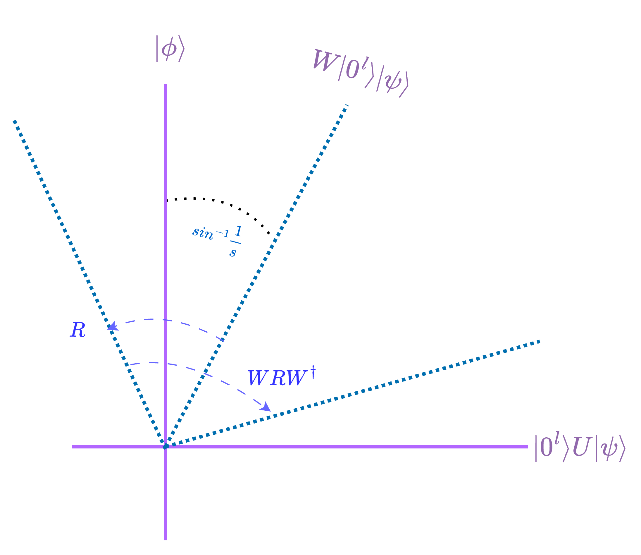
Building the Algorithm with Classiq

image.png

Example: Unitary LCU Amplification

Here we take the matrix A=H0H1=X0+Z02X1+Z12A = H_0\otimes H_1 = \frac{X_0 + Z_0} {\sqrt{2}} \otimes \frac{X_1 + Z_1} {\sqrt{2}} and block-encode it using LCU, creating the matrix UAU_A. In general, though LCU is a combination of unitaries, the result is not necessarily unitary. In this specific example, the matrix AA is unitary, and so the encoding can be amplified using oblivious amplitude amplification.

Block-encoding the Hamiltonian

First show that the sampled state after the application of UAU_A is in the wanted block only in 14\frac {1}{4} of the cases, meaning that in this case s=2s=2. The input ψ|\psi\rangle to UAU_A is a randomly sampled vector of normalized amplitudes.
import numpy as np

from classiq import *

HAMILTONIAN = 0.5 * (
    Pauli.Z(0) * Pauli.X(1)
    + Pauli.X(0) * Pauli.Z(1)
    + Pauli.X(0) * Pauli.X(1)
    + Pauli.Z(0) * Pauli.Z(1)
)


@qfunc
def block_encode(hamiltonian: SparsePauliOp, data: QArray, block: QNum):
    lcu_pauli(hamiltonian, data, block)


@qfunc
def main(data: Output[QNum], block: Output[QNum]):
    allocate(2, block)

    # initialize a random vector
    np.random.seed(1)
    amps = np.random.rand(4)
    amps = (amps / np.linalg.norm(amps)).tolist()
    prepare_amplitudes(amps, 0, data)

    block_encode(HAMILTONIAN, data, block)


qprog = synthesize(main)
result = execute(qprog).result_value()
Print the “good” states:
df = result.dataframe
df[df.block == 0]
datablockcountprobabilitybitstring
3003230.1577150000
4201220.0595700010
810730.0356450001
print("Fraction of `good` states:", df[df.block == 0].probability.sum())
Output:

Fraction of `good` states: 0.2529296875
  

Block-encoding Amplification
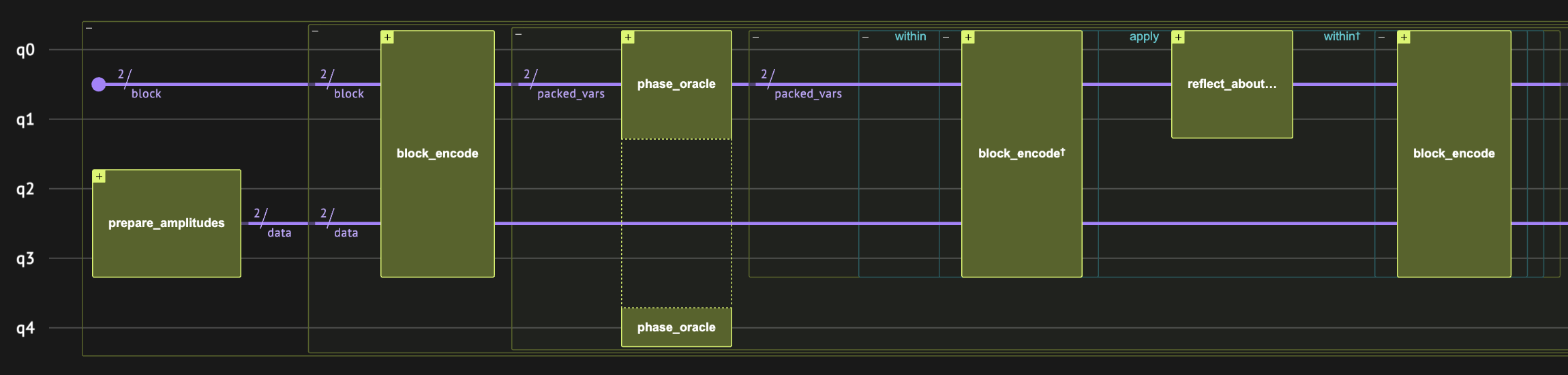
Now we wrap UAU_A with the oblivious amplitude amplification scheme. It is almost like regular Grover, except that it does not take the initial state preparation to the Grover operator. Also, the Grover diffuser only works on the block qubits. (We take advantage of the language capturing mechanism.) The block_oracle (RR in the used notation) operates on the block qubits and checks that they are in the wanted block (i.e., equal to the state 00|00\rangle). The WW operator is represented by the function block_encoding. As the original total amplitude of the “good states” is 12\frac{1}{2}, exactly one Grover iteration will amplify the amplitude to
@qfunc
def oblivious_amplitude_amplification(
    reps: CInt,
    block_encoding: QCallable[QNum, QArray],
    block: QNum,
    data: QArray,
):
    @qperm
    def block_oracle(b: Const[QNum], res: QBit):
        res ^= b == 0

    block_encoding(data, block)
    repeat(
        reps,
        lambda index: grover_operator(
            lambda b: phase_oracle(lambda x, res: block_oracle(x, res), b),
            lambda b: block_encoding(data, b),
            block,
        ),
    )


@qfunc
def main(data: Output[QNum], block: Output[QNum]):
    allocate(2, block)

    # initialize a random vector
    np.random.seed(1)
    amps = np.random.rand(4)
    amps = (amps / np.linalg.norm(amps)).tolist()
    prepare_amplitudes(amps, 0, data)

    oblivious_amplitude_amplification(
        1, lambda _block, _data: block_encode(HAMILTONIAN, _block, _data), block, data
    )


qprog_2 = synthesize(main)
show(qprog_2)
result_2 = execute(qprog_2).result_value()
Output:

Quantum program link: https://platform.classiq.io/circuit/36hZZ6QNxpJsFRG0gj4NNO5sPFr
  

Print the “good” states:
df = result_2.dataframe
df[df.block == 0]
datablockcountprobabilitybitstring
00013530.6606450000
1204560.2226560010
2102390.1166990001
print("Fraction of `good` states:", df.probability.sum())
assert np.isclose(df.probability.sum(), 1)
Output:

Fraction of `good` states: 1.0
  

Extending Where UU is Non-unitary

It was proven that when UU is close to unitary, it is still possible to amplify (using the same operators) and get a good approximation. This is termed “Robust Oblivious Amplitude Amplification” [3]. This is usually the case in Hamiltonian simulation when the LCU reprsents a truncated series which is only an approximation of the unitary eiHte^{-iHt}.

References

[1]: Brassard, Gilles, et al. “Quantum Amplitude Amplification and Estimation.” arXiv preprint quant-ph/0005055 (2000). [2]: Berry, Dominic W., et al. “Exponential improvement in precision for simulating sparse Hamiltonians.” Proceedings of the forty-sixth annual ACM symposium on Theory of Computing (2014). [3]: Berry, Dominic W., et al. “Simulating Hamiltonian dynamics with a truncated Taylor series.” Physical Review Letters 114.9 (2015): 090502.