View on GitHub

Open this notebook in GitHub to run it yourself

Quantum Monte Carlo Integration (QMCI)

Monte Carlo integration refers to estimating expectation values of a function

f(x)

, where

x

is a random variable drawn from some known distribution

p

\begin{equation} \tag{1} E_{p}(x) = \int f(x)p(x) dx. \end{equation}

Such evaluations appear in the context of option pricing or credit risk analysis. The basic idea of QMCI assumes that we have a quantum function

A

, which, for a given

f

and

p

, loads the following state of

n+1

qubits:

\begin{align} \tag{2} A|0\rangle_n|0\rangle = \sum^{2^n-1}_{i=0} \sqrt{f_i} \sqrt{p_i}|i\rangle_n|1\rangle + \sum^{2^n-1}_{i=0} \sqrt{1-f_i} \sqrt{p_i}|i\rangle_n|0\rangle = \sqrt{a}|\psi_1\rangle+\sqrt{1-a}|\psi_0\rangle, \end{align}

where it is understood that the first

2^n

states represent a discretized space of

x

, and that

0\leq f(x)\leq 1

. Then, by applying the amplitude estimation (AE) algorithm for the “good-state”

|\psi_1 \rangle

, we can estimate its amplitude:

a = \sum^{2^n-1}_{i=0} f_i p_i.

The QMCI algorithm can be separated into two parts:

Constructing a Grover operator for the specific problem.

This is done here almost from scratch.

Applying the AE algorithm based on the Grover operator [1].

This is done by calling the Classiq Quantum Phase Estimation (QPE) function.

Specific Use Case for the Tutorial

For simplicity we consider a simple use case. We take a probability distribution on the integers

\tag{3} p_i = \frac{i}{\mathcal{N}} \text{ for } i\in \{0,\dots 2^3-1\},

where

\mathcal{N}

is a normalization constant, and we would like to evaluate the expectation value of the function

\tag{4} f(x) = \sin^2(0.25x+0.2).

Therefore, the value we want to evaluate is

a= \frac{1}{\mathcal{N}} \sum^7_{k=0} \sin^2(0.25k+0.2) k \approx 0.834.

*This tutorial illustrats how to construct a Quantum Monte Carlo Integration (QMCI), defining all its building blocks in Qmod (rather than using open-library functions). The example below demonstrates how we can exploit various concepts of modeling quantum algorithms with Classiq when building our own functions*.

Building the Corresponding Grover Operator

import matplotlib.pyplot as plt

from classiq import *

Grover Operator for QMCI

The Grover operator suitable for QMCI is defined as follows:

Q\equiv - S_{\psi_1} A^{\dagger} S_0 A,

with

S_0

and

S_{\psi_1}

being reflection operators around the zero state

|0\rangle_n|0\rangle

and the good-state

|\psi_1\rangle

, respectively, and the function

A

is defined in Eq. (2). In subsections (1.1)-(1.3) below we build each of the quantum sub-functions, and then in subsection (1.4) we combine them to define a complete Grover operator. On the way we introduce several concepts of functional modeling, which allow the Classiq synthesis engine to reach better optimized circuits.

1.1) The State Loading $A$ Function

We start with constructing the

A

operator in Eq. (2). We define a quantum function and give it the name state_loading. The function’s signature declares two arguments:

A quantum register x declared as QArray (an array of qubits with an unspecified size) that is used to represent the discretization of space.
A quantum register ind of size 1 declared as QBit to indicate the good state.

Next, we construct the logic flow of the state_loading function. The function body consists of two quantum function calls:

As can be seen from Eq. (2), the load_probabilities function is constructed using the Classiq inplace_prepare_state function call on $n=3$ qubits with probabilities $p_i$ .
The amplitude_loading body calls the Classiq linear_pauli_rotations function.

The linear_pauli_rotations loads the amplitude of the function

f(x) = sin^2(0.25 x + 0.2)

. Note: The amplitude should be $sin$ so the probability is $sin^2$ . The function uses an auxiliary qubit that is utilized so that the desired probability reflects on the auxiliary qubit if it is in the |1> state. We use the function with the Pauli Y matrix and enter the appropriate slope and offset to achieve the right parameters. We define the probabilities according to the specific problem described by Eqs. (3-4).

import numpy as np

sp_num_qubits = 3
probabilities = np.linspace(0, 1, 2**sp_num_qubits) / sum(
    np.linspace(0, 1, 2**sp_num_qubits)
)


slope = 0.5
offset = 0.4


@qfunc
def load_probabilities(state: QArray):
    inplace_prepare_state(probabilities.tolist(), 0, state)


@qfunc
def amplitude_loading(x: QArray, ind: QBit):
    linear_pauli_rotations(
        bases=[Pauli.Y.value], slopes=[slope], offsets=[offset], x=x, q=ind
    )


@qfunc
def state_loading(x: QArray, ind: QBit):
    load_probabilities(x)
    amplitude_loading(x=x, ind=ind)

To examine our function we define a quantum main function from which we can build a model, synthesize, and view the quantum program created:

@qfunc
def main(res: Output[QArray[QBit, sp_num_qubits]], ind: Output[QBit]):
    allocate(res)
    allocate(ind)
    state_loading(res, ind)


model = create_model(main)
qprog = synthesize(model)
show(qprog)

Output:

Quantum program link: https://platform.classiq.io/circuit/32pRflos02r3nRujlCT2EAxuz68
  

1.2) $S_{\psi_1}$ Function

The Good State Oracle

The next quantum function we define is the one that reflects around the good state: any

n+1

state in which the ind register is at state

|1\rangle

. This function can be constructed with a ZGate on the ind register.

@qfunc
def good_state_oracle(ind: QBit):
    Z(ind)

1.3) $S_{0}$ Function

The Grover Diffuser

To implement the Grover Diffuser we aim to perform a controlled-Z operation on the

|0>^n

state. We can define a zero_oracle quantum function with the x and ind registers as its arguments. The within_apply operator takes two function arguments—compute and action—and invokes the sequence compute(), action(), and invert(compute()). Quantum objects that are allocated and prepared by compute are subsequently uncomputed and released.

@qfunc
def prepare_minus(q: QBit):
    X(q)
    H(q)


@qfunc
def zero_oracle(x: QNum, ind: QBit):
    within_apply(lambda: prepare_minus(ind), lambda: inplace_xor(x == 0, ind))

The inplace xor operation, ind ^= x==0, is equivalent to control(x==0, X(ind)). We can verify that

\begin{aligned} |00\dots0\rangle \xrightarrow[{\rm ctrl(-Z)(target=q_0, ctrl=q_1\dots q_n)}]{} -|00\dots0\rangle, \\ |10\dots0\rangle \xrightarrow[{\rm ctrl(-Z)(target=q_0, ctrl=q_1\dots q_n)}]{} |10\dots0\rangle, \\ |11\dots0\rangle \xrightarrow[{\rm ctrl(-Z)(target=q_0, ctrl=q_1\dots q_n)}]{} |11\dots0\rangle,\\ |11\dots1\rangle \xrightarrow[{\rm ctrl(-Z)(target=q_0, ctrl=q_1\dots q_n)}]{} |11\dots1\rangle, \end{aligned}

which is exactly the functionality we want.

1.4) $Q$ Function

The Grover Operator

We can now define a complete Grover operator

Q\equiv -S_{\psi_1} A^{\dagger} S_0 A

. We do this in a single code block that calls the following:

The good state oracle (good_state_oracle)
THe inverse of the state preparation (state_loading)
The diffuser (zero_oracle)
The state preparation (state_loading)

Note:

Stages 2-4 are implemented by utilizing the within_apply operator
We add a global phase of -1 to the full operator by using the atomic gate level function U

from classiq.qmod.symbolic import pi


@qfunc
def my_grover_operator(state: QArray):
    good_state_oracle(ind=state[0])
    within_apply(
        lambda: invert(lambda: state_loading(x=state[1 : state.len], ind=state[0])),
        lambda: zero_oracle(state[1 : state.len], state[0]),
    )
    phase(pi)

Let us look at the `my_grover_operator` function we created:

@qfunc
def main(state: Output[QArray[QBit, sp_num_qubits + 1]]):
    allocate(state)
    my_grover_operator(state)


model_2 = create_model(main)
qprog_2 = synthesize(model_2)
show(qprog_2)

Output:

Quantum program link: https://platform.classiq.io/circuit/32pRgqChyKoS2rhIP0zrtt5Gef6
  

Applying Amplitude Estimation (AE) with Quantum Phase Estimation (QPE)

Here we apply a basic AE algorithm that is based on QPE. The idea behind this algorithm is the following: The state

A|0\rangle_n|0\rangle

is spanned by two eigenvectors of our Grover operator

Q

, with the two corresponding eigenvalues

\begin{equation} \tag{5} \lambda_{\pm}=\exp\left(\pm i2\pi \theta \right), \qquad \sin^2 \left(\pi \theta\right)\equiv a. \end{equation}

Therefore, if we apply a QPE on

A|0\rangle_n|0\rangle

, we have these two eigenvalues encoded in the QPE register. However, both give the value of

a

, so there is no ambiguity. To find

a

we build a simple quantum model, applying

A

on a quantum register of size

n+1

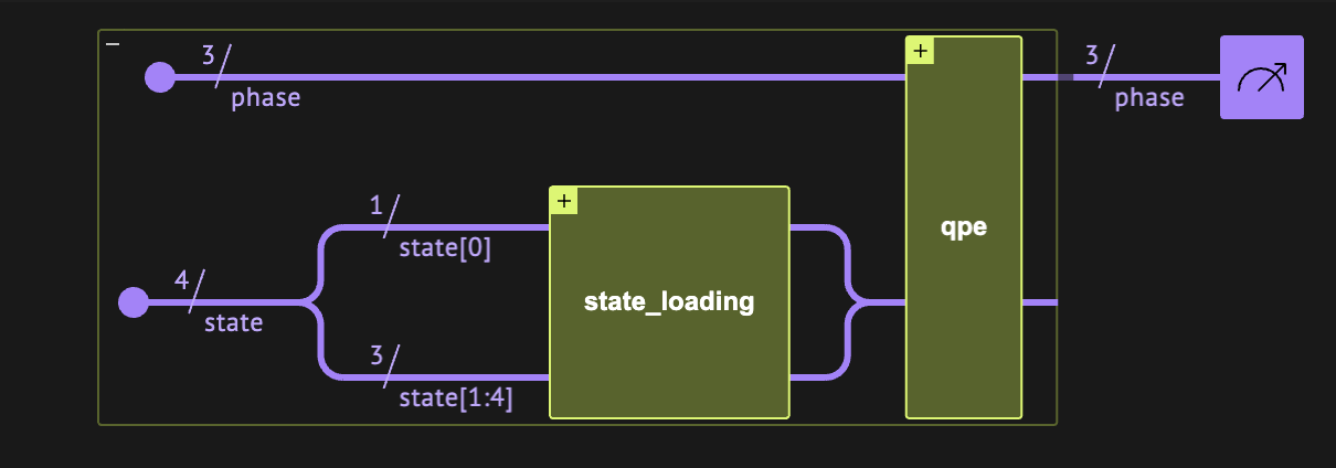
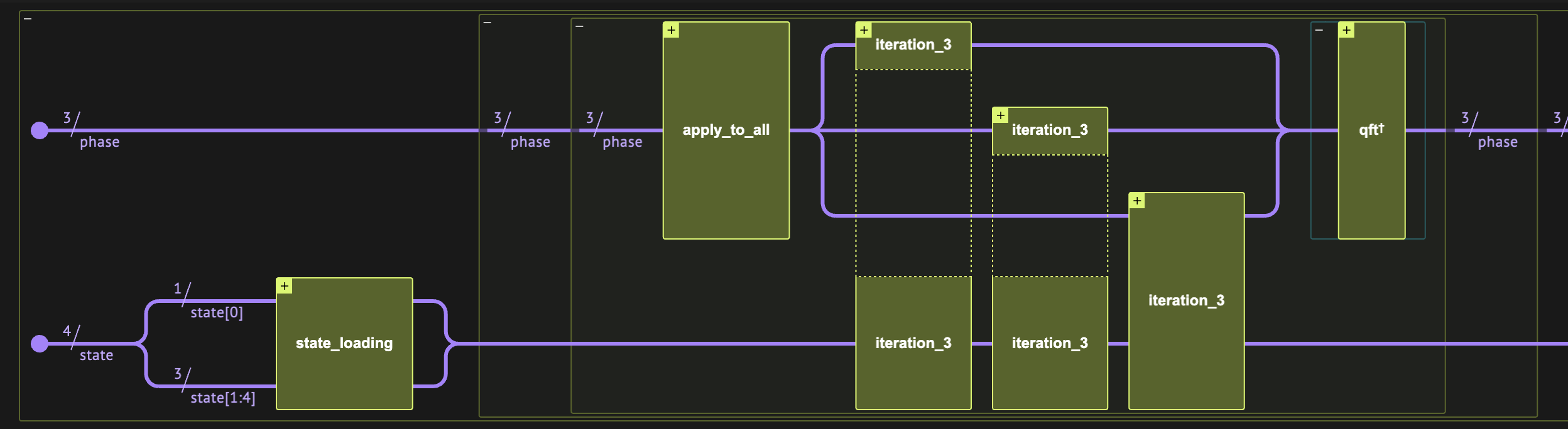
initialized to zero, and then applying the Classiq QPE with the my_grover_operator we defined. Below is the main function from which we can build our model and synthesize it. In particular, we define the output register phase as QNum to hold the phase register output of the QPE. We choose a QPE with phase register of size 3, governing the accuracy of our phase-, and thus amplitude-, estimation.

n_qpe = 3


@qfunc
def main(phase: Output[QNum[n_qpe, SIGNED, n_qpe]]):
    state = QArray()
    allocate(sp_num_qubits + 1, state)
    state_loading(state[1 : state.len], state[0])
    allocate(phase)
    qpe(unitary=lambda: my_grover_operator(state=state), phase=phase)
    drop(state)


model_3 = create_model(main)
model_3 = set_constraints(model_3, Constraints(max_width=9))
qprog_3 = synthesize(model_3)
show(qprog_3)

Output:

Quantum program link: https://platform.classiq.io/circuit/32pRliiRX9wZ3JIgUjvFFezXlPn
  

We can export our model to a .qmod file:

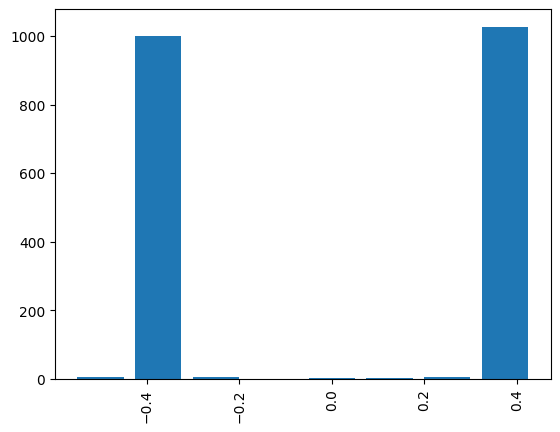
Executing the Circuit and Measuring the Approximated Amplitude

We execute on a simulator:

result = execute(qprog_3).result_value()

## mapping between register string to phases
phases_counts = dict(
    (sampled_state.state["phase"], sampled_state.shots)
    for sampled_state in result.parsed_counts
)

Upon plotting the resulting histogram we see two phase values with high probability (however, both correspond to the same amplitude

a

plt.bar(phases_counts.keys(), phases_counts.values(), width=0.1)
plt.xticks(rotation=90)
print("phase with max probability: ", max(phases_counts, key=phases_counts.get))

Output:

phase with max probability:  0.375

Recalling the relation in Eq. (5), we can read the amplitude

a

from the phase with maximum probability and compare to the expected amplitude:

measured_amplitude = np.sin(np.pi * max(phases_counts, key=phases_counts.get)) ** 2
exact_amplitude = sum(
    np.sin(0.5 * n / 2 + 0.4 / 2) ** 2 * probabilities[n] for n in range(2**3)
)
print(f"measured amplitude: {measured_amplitude}")
print(f"exact amplitude: {exact_amplitude}")

Output:

measured amplitude: 0.8535533905932737
  exact amplitude: 0.8338393824876795
  

assert np.abs(measured_amplitude - exact_amplitude) < 1e-1

References

[1]: [Brassard, G., Hoyer, P., Mosca, M., & Tapp, A. (2002). Quantum Amplitude Amplification and Estimation. Contemporary Mathematics, 305, 53-74.](https://arxiv.org/abs/quant-ph/0005055)

Algorithms

Applications

Functions

Tutorials

Qmc User Defined

View on GitHub

Quantum Monte Carlo Integration (QMCI)

Specific Use Case for the Tutorial

Grover Operator for QMCI

1.1) The State Loading $A$ Function

1.2) $S_{\psi_1}$ Function

1.3) $S_{0}$ Function

1.4) $Q$ Function

Let us look at the `my_grover_operator` function we created:

Executing the Circuit and Measuring the Approximated Amplitude

References

Algorithms

Applications

Functions

Tutorials

View on GitHub

​Quantum Monte Carlo Integration (QMCI)

​Specific Use Case for the Tutorial

​Grover Operator for QMCI

​1.1) The State Loading AAA Function

​1.2) Sψ1S_{\psi_1}Sψ1​​ Function

​1.3) S0S_{0}S0​ Function

​1.4) QQQ Function

​Let us look at the my_grover_operator function we created:

​Executing the Circuit and Measuring the Approximated Amplitude

​References

Quantum Monte Carlo Integration (QMCI)

Specific Use Case for the Tutorial

Grover Operator for QMCI

1.1) The State Loading $A$ Function

1.2) $S_{\psi_1}$ Function

1.3) $S_{0}$ Function

1.4) $Q$ Function

Let us look at the `my_grover_operator` function we created:

Executing the Circuit and Measuring the Approximated Amplitude

References