
View on GitHub

Open this notebook in GitHub to run it yourself

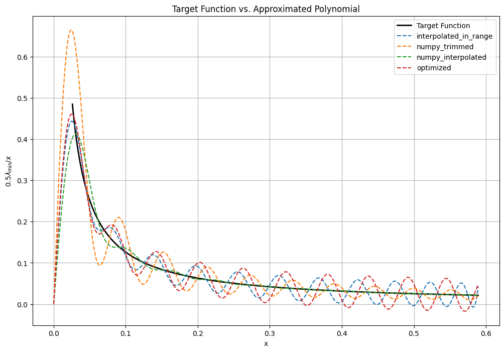
Chebyshev approximation of the inverse function

In this notebook we present the four ways of approximating the inverse function with Chebyshev polynomials:
  1. Using Classiq’s QSP application.
Here the approximation can be made within an interval [\lambda_\min, \lambda_\max], and the polynomial values are bounded in [1,1][-1,1].
  1. Using Numpy interpolation with a give degree, here the polynomial values are bounded in [1,1][-1,1].
  2. Using Numpy interpolation with the theoretical degree, and then trimming to a smaller degree.
  3. Using an optimized (for the Maximum norm) expansion according to https://arxiv.org/pdf/2507.15537 (available in Classiq QSP application).
import matplotlib.pyplot as plt
import numpy as np
from cheb_utils import *
from pauli_be import *
from scipy import sparse

from classiq.applications.chemistry.op_utils import qubit_op_to_qmod

import pathlib

path = (
    pathlib.Path(__file__).parent.resolve()
    if "__file__" in locals()
    else pathlib.Path(".")
)
We upload some matrix, and considered its block-encoding. We need the block-encoding scaling factor in order to calculate the effective range of singular/eigen-values.
mat_name = "nozzle_small_scr"
matfile = "matrices/" + mat_name + ".npz"
mat_raw_scr = sparse.load_npz(path / matfile)
rval = mat_raw_scr.data
col = mat_raw_scr.indices
rowstt = mat_raw_scr.indptr
nr = mat_raw_scr.shape[0]
data_size = int(np.log2(nr))
paulis_list, transform_matrix = initialize_paulis_from_csr(
    rowstt, col, data_size, to_symmetrize=False
)
qubit_op = eval_pauli_op(paulis_list, transform_matrix, rval)
qubit_op.compress(1e-12)
hamiltonian = qubit_op_to_qmod(qubit_op)

be_scaling_factor = sum([np.abs(term.coefficient) for term in hamiltonian.terms])

mat_raw = mat_raw_scr.toarray()

svd = np.linalg.svd(mat_raw / be_scaling_factor)[1]
w_min = min(svd)
w_max = max(svd)
scale = 0.5

degree = 101

print(f"min singular value: {min(svd)}, max_singular value: {max(svd)}")
pcoefs = get_cheb_coeff(
    w_min,
    degree,
    w_max=w_max,
    scale=scale,
    method="interpolated_in_range",
    epsilon=0.01,
)
pcoefs_trimmed = get_cheb_coeff(
    w_min, degree, w_max=w_max, scale=scale, method="numpy_trimmed", epsilon=0.01
)
pcoefs_approx = get_cheb_coeff(
    w_min, degree, w_max=w_max, scale=scale, method="numpy_interpolated", epsilon=0.01
)

pcoefs_optimized = get_cheb_coeff(
    w_min, degree, w_max=w_max, scale=scale, method="optimized", epsilon=0.01
)
Output:
min singular value: 0.02516479472045721, max_singular value: 0.589120855859263
  For error 0.01, and given kappa, the needed polynomial degree is: 899
  Performing convex optimization for the Chebyshev interpolation, with degree 101
  For error 0.01, and given kappa, the needed polynomial degree is: 899
  Performing numpy Chebyshev interpolation, with degree 899 and trimming to degree 101
  For error 0.01, and given kappa, the needed polynomial degree is: 899
  Performing numpy Chebyshev interpolation, with degree 101
  For error 0.01, and given kappa, the needed polynomial degree is: 899
  Taking optimized expansion from literature, with degree 101
  

plot_cheb_inv_approx(
    {
        "interpolated_in_range": pcoefs,
        "numpy_trimmed": pcoefs_trimmed,
        "numpy_interpolated": pcoefs_approx,
        "optimized": pcoefs_optimized,
    },
    w_min,
    w_max,
    scale,
    half_space=True,
)
output