!pip install -qq "classiq[qsp]"
!pip install -qq "classiq[chemistry]"

import time

import matplotlib.pyplot as plt
import numpy as np
from banded_be import get_banded_diags_be
from cheb_utils import *
from classical_functions_be import get_projected_state_vector, get_svd_range
from pauli_be import get_pauli_be
from scipy import sparse

from classiq import *

np.random.seed(53)

PAULI_TRIM_REL_TOL = 0.1

from classiq.qmod.symbolic import pi


@qfunc
def my_reflect_about_zero(qba: QNum):
    control(qba == 0, lambda: phase(pi))
    phase(pi)


@qfunc
def walk_operator(
    block_enc: QCallable[QArray, QArray], block: QArray, data: QArray
) -> None:
    block_enc(block, data)
    my_reflect_about_zero(block)


@qfunc
def symmetrize_walk_operator(
    block_enc: QCallable[QNum, QArray], block: QNum, data: QArray
):
    my_reflect_about_zero(block)
    within_apply(
        lambda: block_enc(block, data),
        lambda: my_reflect_about_zero(block),
    )


@qfunc
def lcu_cheb(
    powers: CArray[CInt],
    inv_coeffs: CArray[CReal],
    block_enc: QCallable[QNum, QArray],
    mat_block: QNum,
    data: QArray,
    cheb_block: QArray,
) -> None:

    within_apply(
        lambda: inplace_prepare_state(inv_coeffs, 0.0, cheb_block),
        lambda: (
            Z(cheb_block[0]),
            repeat(
                powers.len,
                lambda i: control(
                    cheb_block[i],
                    lambda: power(
                        powers[i],
                        lambda: symmetrize_walk_operator(block_enc, mat_block, data),
                    ),
                ),
            ),
            my_reflect_about_zero(mat_block),
            walk_operator(block_enc, mat_block, data),
        ),
    )

def cheb_lcu_solver(
    mat_raw_scr,
    b_raw,
    log_poly_degree,
    be_method="banded",
    cheb_approx_type="numpy_interpolated",
    preferences=Preferences(),
    constraints=Constraints(),
):

    SCALE = 0.5
    b_norm = np.linalg.norm(b_raw)  # b normalization
    b_normalized = b_raw / b_norm
    data_size = max(1, (len(b_raw) - 1).bit_length())

    # Define block encoding
    if be_method == "pauli":
        data_size, block_size, be_scaling_factor, be_qfunc = get_pauli_be(mat_raw_scr)
    if be_method == "banded":
        data_size, block_size, be_scaling_factor, be_qfunc = get_banded_diags_be(
            mat_raw_scr
        )

    # Get eigenvalues range
    w_min, w_max = get_svd_range(mat_raw_scr / be_scaling_factor)
    # Calculate approximated Chebyshev polynomial
    poly_degree = 2 * (2**log_poly_degree - 1) + 1
    pcoefs, poly_scale = get_cheb_coeff(
        w_min,
        poly_degree,
        w_max,
        scale=SCALE,
        method=cheb_approx_type,
        epsilon=0.01,
    )
    odd_coef = pcoefs[1::2]
    # Calculate prep for Chebyshev LCU
    lcu_size_inv = len(odd_coef).bit_length() - 1
    print(f"Chebyshec LCU size: {lcu_size_inv} qubits.")
    odd_coeffs_signs = np.sign(odd_coef)
    assert np.all(
        odd_coeffs_signs == np.where(np.arange(len(odd_coeffs_signs)) % 2 == 0, 1, -1)
    ), "Non alternating signs for odd coefficients"
    normalization_inv = sum(np.abs(odd_coef))
    print(f"Normalization factor for inversion: {normalization_inv}")
    prepare_probs_inv = (np.abs(odd_coef) / normalization_inv).tolist()

    @qfunc
    def main(
        matrix_block: Output[QNum[block_size]],
        data: Output[QNum[data_size]],
        inv_block: Output[QNum[lcu_size_inv]],
    ):

        allocate(inv_block)
        allocate(matrix_block)
        prepare_amplitudes(b_normalized.tolist(), 0, data)

        lcu_cheb(
            powers=[2**i for i in range(lcu_size_inv)],
            inv_coeffs=prepare_probs_inv,
            block_enc=lambda b, d: invert(lambda: be_qfunc(b, d)),
            mat_block=matrix_block,
            data=data,
            cheb_block=inv_block,
        )

    start_time_syn = time.time()
    qprog = synthesize(main, preferences=preferences, constraints=constraints)

    print("time to syn:", time.time() - start_time_syn)

    execution_preferences = ExecutionPreferences(
        num_shots=1,
        backend_preferences=ClassiqBackendPreferences(
            backend_name=ClassiqSimulatorBackendNames.SIMULATOR_STATEVECTOR
        ),
    )

    start_time_exe = time.time()
    with ExecutionSession(qprog, execution_preferences) as es:
        es.set_measured_state_filter("matrix_block", lambda state: state == 0.0)
        es.set_measured_state_filter("inv_block", lambda state: state == 0.0)
        results = es.sample()
    print("time to exe:", time.time() - start_time_exe)

    resulting_state = get_projected_state_vector(results, "data")

    normalization_factor = (be_scaling_factor * poly_scale) / b_norm / normalization_inv

    return resulting_state / normalization_factor, qprog

import pathlib

path = (
    pathlib.Path(__file__).parent.resolve()
    if "__file__" in locals()
    else pathlib.Path(".")
)

mat_name = "nozzle_small_scr"
matfile = "matrices/" + mat_name + ".npz"
mat_raw_scr = sparse.load_npz(path / matfile)

b_raw = np.load(path / "matrices/b_nozzle_small.npy")
raw_mat_qubits = len(b_raw).bit_length() - 1  # matrix raw size

print(f"Raw matrix size: {raw_mat_qubits} qubits.")

# For faster results use the commented out preferences

prefs = Preferences()

# prefs = Preferences(
#     transpilation_option="none", optimization_level=0, debug_mode=False, qasm3=True
# )

log_poly_degree = 5

qsol_banded, qprog_cheb_lcu_banded = cheb_lcu_solver(
    mat_raw_scr,
    b_raw,
    log_poly_degree,
    be_method="banded",
    preferences=prefs,
    constraints=Constraints(optimization_parameter="width"),
)
show(qprog_cheb_lcu_banded)

qsol_pauli, qprog_cheb_lcu_pauli = cheb_lcu_solver(
    mat_raw_scr,
    b_raw,
    log_poly_degree,
    be_method="pauli",
    preferences=prefs,
    constraints=Constraints(optimization_parameter="width"),
)
show(qprog_cheb_lcu_pauli)

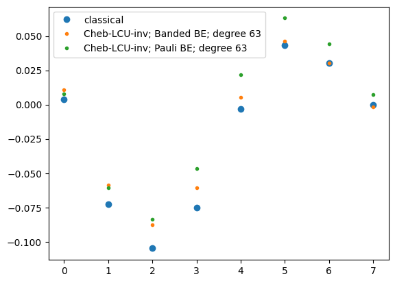
mat_raw = mat_raw_scr.toarray()
expected_sol = np.linalg.solve(mat_raw, b_raw)
plt.plot(expected_sol, "o", label="classical")
ext_idx = np.argmax(np.abs(expected_sol))
correct_sign = np.sign(expected_sol[ext_idx]) / np.sign(qsol_banded[ext_idx])
qsol_banded *= correct_sign
plt.plot(
    qsol_banded,
    ".",
    label=f"Cheb-LCU-inv; Banded BE; degree {2*2**log_poly_degree-1}",
)
correct_sign = np.sign(expected_sol[ext_idx]) / np.sign(qsol_pauli[ext_idx])
qsol_pauli *= correct_sign
plt.plot(
    qsol_pauli,
    ".",
    label=f"Cheb-LCU-inv; Pauli BE; degree {2*2**log_poly_degree-1}",
)
plt.legend()

assert np.linalg.norm(qsol_banded[0 : len(b_raw)] - expected_sol) < 0.25
assert np.linalg.norm(qsol_pauli[0 : len(b_raw)] - expected_sol) < 0.2